For image classification tasks, a common choice for convolutional neural network (CNN) architecture is repeated blocks of convolution and max pooling layers, followed by two or more densely connected layers. The final dense layer has a softmax activation function and a node for each potential object category.

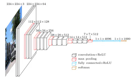
As an example, consider the VGG-16 model architecture, depicted in the figure below.

We can summarize the layers of the VGG-16 model by executing the following line of code in the terminal:

python -c 'from keras.applications.vgg16 import VGG16; VGG16().summary()'

Your output should appear as follows:

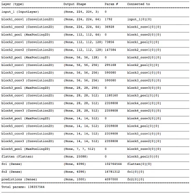
You will notice five blocks of (two to three) convolutional layers followed by a max pooling layer. The final max pooling layer is then flattened and followed by three densely connected layers. Notice that most of the parameters in the model belong to the fully connected layers!

As you can probably imagine, an architecture like this has the risk of overfitting to the training dataset. In practice, dropout layers are used to avoid overfitting.

Global Average Pooling

In the last few years, experts have turned to global average pooling (GAP) layers to minimize overfitting by reducing the total number of parameters in the model. Similar to max pooling layers, GAP layers are used to reduce the spatial dimensions of a three-dimensional tensor. However, GAP layers perform a more extreme type of dimensionality reduction, where a tensor with dimensions $h \times w \times d$ is reduced in size to have dimensions $1 \times 1 \times d$. GAP layers reduce each $h \times w$ feature map to a single number by simply taking the average of all $hw$ values.

The first paper to propose GAP layers designed an architecture where the final max pooling layer contained one activation map for each image category in the dataset. The max pooling layer was then fed to a GAP layer, which yielded a vector with a single entry for each possible object in the classification task. The authors then applied a softmax activation function to yield the predicted probability of each class. If you peek at the original paper, I especially recommend checking out Section 3.2, titled “Global Average Pooling”.

The ResNet-50 model takes a less extreme approach; instead of getting rid of dense layers altogether, the GAP layer is followed by one densely connected layer with a softmax activation function that yields the predicted object classes.

Object Localization

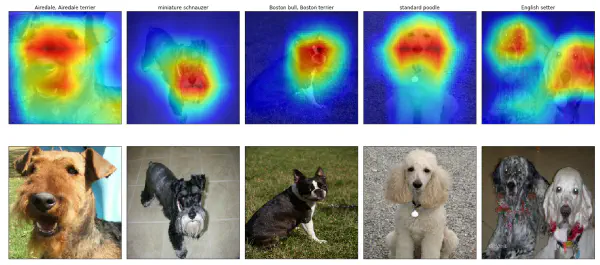
In mid-2016, researchers at MIT demonstrated that CNNs with GAP layers (a.k.a. GAP-CNNs) that have been trained for a classification task can also be used for object localization. That is, a GAP-CNN not only tells us what object is contained in the image - it also tells us where the object is in the image, and through no additional work on our part! The localization is expressed as a heat map (referred to as a class activation map), where the color-coding scheme identifies regions that are relatively important for the GAP-CNN to perform the object identification task. Please check out the YouTube video below for an awesome demo!

In the repository, I have explored the localization ability of the pre-trained ResNet-50 model, using the technique from this paper. The main idea is that each of the activation maps in the final layer preceding the GAP layer acts as a detector for a different pattern in the image, localized in space. To get the class activation map corresponding to an image, we need only to transform these detected patterns to detected objects.

This transformation is done by noticing each node in the GAP layer corresponds to a different activation map, and that the weights connecting the GAP layer to the final dense layer encode each activation map’s contribution to the predicted object class. To obtain the class activation map, we sum the contributions of each of the detected patterns in the activation maps, where detected patterns that are more important to the predicted object class are given more weight.

How the Code Operates

Let’s examine the ResNet-50 architecture by executing the following line of code in the terminal:

python -c 'from keras.applications.resnet50 import ResNet50; ResNet50().summary()'

The final few lines of output should appear as follows (Notice that unlike the VGG-16 model, the majority of the trainable parameters are not located in the fully connected layers at the top of the network!):

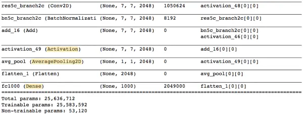
The Activation, AveragePooling2D, and Dense layers towards the end of the network are of the most interest to us. Note that the AveragePooling2D layer is in fact a GAP layer!

We’ll begin with the Activation layer. This layer contains 2048 activation maps, each with dimensions $7\times7$. Let $f_k$ represent the $k$-th activation map, where $k \in {1, \ldots, 2048}$.

The following AveragePooling2D GAP layer reduces the size of the preceding layer to $(1,1,2048)$ by taking the average of each feature map. The next Flatten layer merely flattens the input, without resulting in any change to the information contained in the previous GAP layer.

The object category predicted by ResNet-50 corresponds to a single node in the final Dense layer; and, this single node is connected to every node in the preceding Flatten layer. Let $w_k$ represent the weight connecting the $k$-th node in the Flatten layer to the output node corresponding to the predicted image category.

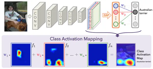
Then, in order to obtain the class activation map, we need only compute the sum

$$w_1 \cdot f_1 + w_2 \cdot f_2 + \ldots + w_{2048} \cdot f_{2048}.$$

You can plot these class activation maps for any image of your choosing, to explore the localization ability of ResNet-50. Note that in order to permit comparison to the original image, bilinear upsampling is used to resize each activation map to $224 \times 224$. (This results in a class activation map with size $224 \times 224$.)

If you’d like to use this code to do your own object localization, you need only download the GitHub repository.